This is the english translation version of this page.
Since I am not powerful enough to translate it at once, I will gradually
translate it. So, for a while, you will find this page in partially translated to
English from Japanese. English is very difficult language.
People who can read/write ENGLISH freely should be genius!
By the way, the method is based on my master thesis done over 30 years ago. On those days, while I thought we could do it, I have not done till now. 5 years ago, I retired a company, I tried it again, and I dit it very easily. As I said, it contains something cheat. If I exipress the situation rigorously, I only got up to arrange the segments of the solution linearly.
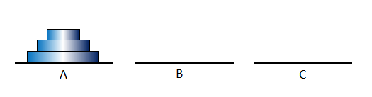
The problem is to find the sequence to move all the disks to B, one by one. All the disks are different sizes, and we cannot place a larger disk on a smaller disk. Under the constraint, we are asked to move all the disks to the place B.
To solve this problem, firstly, we move n-1 disks over the largest disk to the place C, move the largest disk n from A to B, finally, move n-1 disks at the place C to the place B. The following program written in the language 'ruby' is an implementation this method.
defhanoi(n, a, b, c) if (n == 0) # do nothing elsehanoi(n-1, a, c, b) printf("Move disk %d from %s to %s\n", n, a, b)hanoi(n-1, c, b, a) end end hanoi(3, "A", "B", "C")
When you call the function as the last line, the following solution will be shown. The feature of recursive call is very convenient.
  Move disk 1 from A to B
  Move disk 2 from A to C
  Move disk 1 from B to C
  Move disk 3 from A to B
  Move disk 1 from C to A
  Move disk 2 from C to B
  Move disk 1 from A to B
Although this program is easy to understand for human, since it uses printf() which has a side-effect, we modify the program to return whole the sequence without side effects. We use the global variable $clount1 to count the number of recursive calls.
defhanoi(n, a, b, c) $count1 = 0hanoi1(n, a, b, c) end defhanoi1(n, a, b, c) $count1 += 1 if (n == 0) [] elsehanoi1(n-1, a, c, b) + ["Move disk " + n.to_s + " from " + a + " to " + b] +hanoi1(n-1, c, b, a) end end hanoi(3, "A", "B", "C")
This produces the following result.
 ["Move disk 1 from A to B", "Move disk 2 from A to C",
  "Move disk 1 from B to C", "Move disk 3 from A to B",
  "Move disk 1 from C to A", "Move disk 2 from C to B",
  "Move disk 1 from A to B"]
The count of the recursive calls $count1 is 15.
When we choose C(n) the number of call to hanoi() as a measure of the complexity,
  C(0) = 1
  C(n+1) = 2*C(n) + 1
hence
  C(n) = 2n+1 - 1
the complexiy is O(2n).
In the following, we improve so that the order of recursive calls become O(n).
But, the task of appending arrays [...] + [...] to construct the solution
requires the time proposional to
the length of the former array, the complexity remains still O(2n).
It is very regrettable...
$memo[[n, a, b, c]] = result
and, use $memo[[n, a, b, c]] if it has some value.
defhanoi2(n, a, b, c) $memo = {} # We use an association list to memoize the result of # computations $count2 = 0hanoi2b(n, a, b, c) end defhanoi2b(n, a, b, c) $count2 += 1 result = $memo[[n, a, b, c]] if result != nil then return result end if (n == 0) result = [] else result =hanoi2b(n-1, a, c, b) + ["Move disk " + n.to_s + " from " + a + " to " + b] +hanoi2b(n-1, c, b, a) end $memo[[n, a, b, c]] = result result end # Since if we print the result, it requires a lot of time, # we will do as follows. xxx=hanoi2(10, "A", "B", "C") ; nil $count2 # The number of calls to hanoi2() 55 xxx.length # The length of the solution 1023 # 2**10 - 1 = 1023 correct answer xxx==hanoi(10, "A", "B", "C") true # The result is surely correct
In this example, the number of recursive calls to hanoi2() is 55 when n=10. Since the original program requires 211-1=2047 times, the load to the recursive calls is lowered. However the work to concatenate arrays is big. In my computer, the program rapidly be slower when n is larger than 20, and could not complete the task for n=30 (I stopped the program on the way). Consider that the length of the solution is 230 - 1 = 1,073,741,823 when n=30. Because I retired earlier than the usual retirement year, I am poor enough not to be able to buy a new computer.
To improve this program to O(n) program, you can proceed to "4. Consideration on appending arrays". But, I have an interest on the other method using program transformation, I am glad if you also read the next section "3.2 Program transformation with tupling strategy", later.
Since it will time consuming to explain very first, we put the following auxiliary function without reasons (See comment1).
    def hanoi_triple(n, a, b, c)
      [hanoi(n, a, b, c), hanoi(n, b, c, a), hanoi(n, c, a, b)]
    end
Then, the function call
If this triple has been computed, the original triple:(*) [hanoi(n-1, a, c, b), hanoi(n-1, c, b, a), hanoi(n-1, b, a, c)]
can be easily computed. For example, the first term of (**) can be computed by values of the first term and the second term of (*) using the first definition of hanoi(). We will check the second term of (*), i.e., hanoi(n, b, c, a) can be computed similarly.(**) [hanoi(n, a, b, c), hanoi(n, b, c, a), hanoi(n, c, a, b)]
Please check the third of (**) is computed by the values in (*) by yourself.hanoi(n, b, c, a) (i.e., to move n disks from b to c) would be done by moving n-1 disks from b to a (hanoi(n-1, b, a, c), the third term of (*)), move the disk n from b to c directly, moving n-1 disks from a to c (hanoi(n-1, a, c, b), the first term of (*))
By noticing the fact above, we can rewrite hanoi_triple() as follows so that it call itself only once.
# hanoi_triple(n, a, b, c) is intended to compute # [hanoi(n, a, b, c), hanoi(n, b, c, a), hanoi(n, c, a, b)] defhanoi3(n, a, b, c) $count3 = 0hanoi_triple(n, a, b, c) [0] end defhanoi_triple(n, a, b, c) $count3 += 1 if n == 0 then [[], [], []] else x =hanoi_triple(n-1, a, c, b) [x[0] + ["Move disk " + n.to_s + " from " + a + " to " + b] + x[1], x[2] + ["Move disk " + n.to_s + " from " + b + " to " + c] + x[0], x[1] + ["Move disk " + n.to_s + " from " + c + " to " + a] + x[2]] end end yyy=hanoi3(10, "A", "B", "C") ; nil $count3 # 11 times recursive call 11 yyy==hanoi(10, "A", "B", "C") true # the answer is correct.
I studied how to introduce such auxiliary function systematically for my master thesis, 1983-1984. The description was very complex, had many typos and was hard to read. So, I explained it in the appendix of this page simplifying by loosing its generality a little.
There are many representation of array (or list too). For example, in the logic-based language Prolog, some people used so called 'difference list' which represents a list by a pair of lists. The difference between its component lists represents the original list. The difference list can be concatenated very efficiently.
Considering such techniques, I thought that the result do not have to be represented as a concrete array. The result may be represented by something that can be interpreted as 'the result' essentially. In the solution of Hanoi problem, same sequences of moving actions appear many times. There may be some methods to share those same sequences and represent the long solution very compactly.
To tell the conclusion, I could not invent such a ingenious linked structure, since a same sequence is used in many contexts.
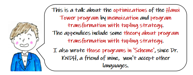
Therefore, as the second idea, I thought the following convention.
That is, if an element of an array is an array beginning with *expand*, we think the element is a sequence of elements expanded there.
Further, we can omit also *expand* with the convention to think an array which has several depth arrays as it elements to be a single flat array of their elements.
Thus, I put the convention:
Convention:
  An array
    [X1, X2, [Y1, Y2, Y3], X3, X4]
  represents the flat array
    [X1, X2, Y1, Y2, Y3, X3, X4]
Then the memoization version would become to the following programs.
defhanoi2(n, a, b, c) $memo = {} # We use an association list to memoize the result of # computations $count2 = 0hanoi2b(n, a, b, c) end defhanoi2b(n, a, b, c) $count2 += 1 result = $memo[[n, a, b, c]] if result != nil then return result end if (n == 0) result = [] else # point is to give up appending arrays and to return the # list of 3 elements result = [hanoi2b(n-1, a, c, b) , "Move disk " + n.to_s + " from " + a + " to " + b,hanoi2b(n-1, c, b, a) ] end $memo[[n, a, b, c]] = result result end # While the next result seems a little complex, you would understand # the solution is given by tracing "Move disk ..." parts. xxx=hanoi2(3, "A", "B", "C") [[[[], "Move disk 1 from A to B", []], "Move disk 2 from A to C", [[], "Move disk 1 from B to C", []]], "Move disk 3 from A to B", [[[], "Move disk 1 from C to A", []], "Move disk 2 from C to B", [[], "Move disk 1 from A to B", []]]] # This version requires only 595 recursive calls for 100 disks xxx=hanoi2(100, "A", "B", "C") ; nil $count2 595
We will translate the program transformation version in this form.
defhanoi3(n, a, b, c) $count3 = 0hanoi_triple(n, a, b, c) [0] end defhanoi_triple(n, a, b, c) $count3 += 1 if n == 0 then [[], [], []] else x =hanoi_triple(n-1, a, c, b) [[x[0], "Move disk " + n.to_s + " from " + a + " to " + b, x[1]], [x[2], "Move disk " + n.to_s + " from " + b + " to " + c, x[0]], [x[1], "Move disk " + n.to_s + " from " + c + " to " + a, x[2]]] end endhanoi3(3, "A", "B", "C") [[[[], "Move disk 1 from A to B", []], "Move disk 2 from A to C", [[], "Move disk 1 from B to C", []]], "Move disk 3 from A to B", [[[], "Move disk 1 from C to A", []], "Move disk 2 from C to B", [[], "Move disk 1 from A to B", []]]] # Even if n=1000, the computation is easily done. # The length of the sequence is 21000 - 1hanoi3(1000, "A", "B", "C") ; nil $count3 1001
Although the value of the following information is doubtful, the length of the sequence of moving action for n=1000 is
  21000 - 1 =
10715086071862673209484250490600018105614048117055
33607443750388370351051124936122493198378815695858
12759467291755314682518714528569231404359845775746
98574803934567774824230985421074605062371141877954
18215304647498358194126739876755916554394607706291
45711964776865421676604298316526243868372056680693
75
a number of 302 digits( 50 digits/line).
I will remove unsightly empty arrays in the result.
defhanoi3(n, a, b, c) $count3 = 0hanoi_triple(n, a, b, c) [0] end defhanoi_triple(n, a, b, c) $count3 += 1 if n == 1 then ["Move disk " + n.to_s + " from " + a + " to " + b, "Move disk " + n.to_s + " from " + b + " to " + c, "Move disk " + n.to_s + " from " + c + " to " + a] else x =hanoi_triple(n-1, a, c, b) [[x[0], "Move disk " + n.to_s + " from " + a + " to " + b, x[1]], [x[2], "Move disk " + n.to_s + " from " + b + " to " + c, x[0]], [x[1], "Move disk " + n.to_s + " from " + c + " to " + a, x[2]]] end endhanoi3(3, "A", "B", "C") [["Move disk 1 from A to B", "Move disk 2 from A to C", "Move disk 1 from B to C"], "Move disk 3 from A to B", ["Move disk 1 from C to A", "Move disk 2 from C to B", "Move disk 1 from A to B"]]
I think we are face to the question "What is a computation? Is the proposed solution is really a solution to the original problem?".
(Frankly speaking, the following japanese paragraphs says the above).
ここではメモ化やプログラム変換を使って,ハノイの塔のプログラムを
円盤数 n に対して,リニアなオーダーの再帰呼び出しで解くプログラムに
改善する方法を述べた.また,解のデータ構造を改善して,実際の計算時間も
リニアになるように工夫した.
しかし,ここで読者には疑問というか不満があるに違いない.「本来,
解は線形の配列(またはリスト)で表現されていたのに,ここでやった
ようにかなり深くネストして表現されていて良いのだろうか?」と.
これを人の目に分かりやすく見せるためには,配列のネストを解いて,
一次元に並べる必要があり,その作業を残して,解を得たと言えるのだろうか.
まだ,解答の途中なのではないだろうかと.
実は私もこれは疑問のままである.例えば,遅延評価の機構を持った
言語でハノイの塔を普通に再帰的に解くと,まったく具体的な計算を行わずに
計算が終わり,結果の中の,例えば3番目の移動操作を調べに行ったところで
始めて必要な計算がなされ,その移動操作がユーザに提示される.
このとき,最初の解を求めるプログラムの計算量は O(1) と言えるのだろうか?
今回提示した解でのネストを許したものが解と言えるなら,こちらも
解と言えるような気もする.違うところがあるとするなら,我々がやった方は,
今回の実験や考察は,「計算」というものに対する何か深遠なるものを
我々に投げかけているような気もするし,案外,たわいもない話なのかもしれない.
もしかしたら.この問題で求められるものが何かということがぶれているだけの
ことかもしれない.
くらいである.
私の( Akihiko Koga) も, 探したら PDF が見つかったのでリンクを貼っておく.かなり煩雑なのとタイポが あるので,ここの付録で簡単に解説した.
We studied the method of introducing an auxiliary function for tupleing strategy (semi-)automatically.
The program transformation in this page is based on the method of my paper:
Akihiko, Koga : On Program Transformation with Tupling Technique, RIMS Symposia on Software Science and Engineering ||, 1983 and 1984: Kyoto, Japan, Lecture Notes in Computer Science 220, 1985, pp. 212-232Although it is strange to say by myself, the paper is very cumbersome and it also contains a lot of typos. Since the target programs of the transformation are mutual recursive ones, many function symbols appeared, terms were subscripted two times, and the whole description became very complex.
Therefore, here we are going to explain the simplified version of the paper by constraining our target program to have only a single function symbol.
Because people who read this article would know what program transformation is, I put the background chapter to the last position. If you are not aquainted with it, please read there first.
As we have already said, we only handle programs with one symbol function.
We do not spesify any concrete programming language. We use some
functional language-like informal programming language with common
vague understanding. The language contains
Our target program is of the following form (<= means the left hand-side is defined by the right hand-side).
  f(x) <= Φ(f(σ1(x)), ..., f(σn(x)))

	Here Φ(...) is a expression which is composed of function
        application, conditional statements by 'if', etc.
	σ1, ..., σn are somewhat known functions to operate on
        the variable x.
Here, while we constrain the function to be defined
The following
 fib(n) <= if (n=0 or n=1) then 1 else fib(n-1) + fib(n-2) end

         Here, suppose the syntax of our target programs has
                if ... then ... else ... end
         structure,and it has common meaning.
Here, σ1, ..., σn in this example are
σ1 = λn.n-1Here, λx.Φ(x) is a notation of function which has one parameter x and returns the value Φ(x). This notation is called
σ2 = λn.n-2 = σ1·σ1=σ12
Using the very rough scheme, this example is expressed as follows .
fib(n) = Φ(fib(σ1(n) ), fib(σ12(n)) )
This very rough scheme expresses the
In the next chapter, we formulate the problem to find an appropriate tuple for the program transformation to the dependency of a given recursive program.{σ1,σ12}
By the way, when we rewrite the Fibonacci number program as follows, we get O(n) order program of Fibonacci number program while the original program require exponential computation to n.
fib(n) <= u where [u, v] =fib_pair(n) fib_pair(n) <= if (n = 0 or n = 1) then [1, 1] else [u+v, u] where [u, v] =fib_pair(n-1) end Here,[u, v] is the tuple of value u and v. The statementu where [u, v] = fib_pair(n) means that first, we compute fib_pair(n) and set the result to [u, v] and under the binding of variables u and v, return u. The 'where' clause in fib_pair(n) expresses similar meaning.
The call graph of the both definitions are explained in the Background chapter.
We formulate the problem "For the dependency of a given program, we find an appropriate tuple candidate for the smooth program transformation with tupling strategy".
For the program
f(x) <= Φ(f(we call the set of functionsσ1(x) ), ..., f(σn(x) ))
the{σ1, ..., σn}
In the following, we combine the functions applied to f's argument, i.e.,
σ1, ..., σn and seek for the candidate of the tuple
for program transformation. Therefore, it is valuable to consider the
space of such functions. Such space is called a
If each element x of M has its inverse x-1 such that
x·x-1 = x-1·x = e
M is called a
In the discussion below, the monoid M, the space of functions that includes functions in a dependency, is chosen appropriately. Usually, M := [D], which means the monoid generated by elements of D (the smallest monoid that include all elements of D). M can be an infinite set. For example, suppose D := {λn.n-1}. In this case,
M := [D] = {λn.n-a | a is an integer}
which is equivalent to the monoid of the integers Z with the usual addition as its operation.
We define some notations about monoids.
Let M be a monoid of functions generated by the functions appearing in a given program and σ, ρ ∈ M,A, B ⊆ M, n be an integer ≤ 0.
Caution: Sometimes, we use A·B, σ·A instead of AB, σA, when some ambiguity may occur or we want to enphasize the operation.
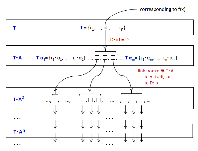
Lastly, we define the concepts (c-tuple, linear c-tuple) intended as a tuple that expresses the auxiliary function introduced for the program transformation with tupling strategy.
Let D = {σ1, ..., σn} be a dependency and M be a monoid such that D ⊆ M.
A pair of A ⊆ M and T ⊆ M ,
'c-tuple' is a short for a Candidate for a tuple.
Since the case of |A| = 1 is very important, we call such c-tuple
Suppose that a c-tuple (A, T) is found for a given dependency D. The figure 2.1 shows the relationships among elements in T, Tα for α∈A. τ∈T satisfies either of the conditions.
This means that all the elements of T can be expressed using the elements in Tα1, ..., Tαm according to the relation in the dependency D.
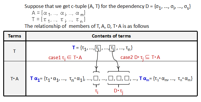
c-tuple (A, T) is intended as an auxiliary function to be introduced for the program transformation.
Let A = {α1, ..., αm}, the auxiliary function h(x) may be expressed recursively with some description Φ
Of cource, we need, say, if statements in Φ to ensure the termination of the computation.
From the intention of the rewritten above, it is not good that we get id combining elements of A. It means cyclic computation. Therefore, we set the third condition
The following japanese paragraph are some comments about
c-タプル (A, T) が見つかったとする.しかし,読者は,このような
プログラムの書き換えを行ったとき,引数に対する色々な関数適用の組み合わせがなされ,
元の定義では呼び出されなかった引数の値に対して計算が要求されるかもしれない
という心配を持つかもしれない.これは妥当な心配であるが,当面は,記述 Φ を
うまく行うことによって
c-タプルの中で,A が唯一の要素からなるとき(singleton set であるとき)は,
1つだけの再帰呼び出ししか持たない再帰関数に変換できる可能性があると
いうことであり,特に重要である.この場合は,もとの指数関数的な計算量が
線形のオーダーの計算量になる
可能性がある.この場合の c-タプルを,
Example
The dependency of Fibonacci number program is D = {σ, σ2}.
Here, σ=λn.n-1. The following is a linear c-tuple of D.
We introduce the following auxiliary function according to the linear c-tuple.(A, T) = ({σ}, {id, σ})
fib_pair(n) = [fib(id(n)), fib(σ(n))] = [fib(n), fib(n-1)]
This function can be expressed using
  fib(n) <= u where [u, v] = fib_pair(n)
  fib_pair(n) <= if n < 2 then [1, 1]
                 else
                   [u+v, u] where [u, v] = fib_pair(n-1)
                 end
In this example, time complexity is improved from exponetial to linear of n.
In this chapter, we state some theorems that express knowhows to find c-tuples for a given dependency, e.g., "When a linear c-tuple exists?", "How we can reduce the dependency to simple ones?", etc.
Let D be a dependency. If
|∪ i=0 to s Di| / s →∞ (as s →∞)
there is no linear c-tuple.
[Proof [to be translate later]] この依存性 D にリニア c-タプル ({α}, T) が存在したとする. |T| = B とするとき,s ≥ 0 に対して, Ds ⊆ ∪i = 0 to B·s(T·αi) が s に関する帰納法で証明することができる. したがって,D にリニア c-タプルがあれば, ∪ i=0 to s Di ⊆ ∪i = 0 to B·s(T·αi) となりる.右辺の集合のサイズは,高々 |T|·s·B にしかならないので, ∪ i=0 to s Di は,高々,s に対して線形でしか大きくならない.[Q.E.D.]
The combination of m objects in n objects, C(n, m) can be obtained by the following recurrent formula
    C(n, m) = C(n-1, m-1) + C(n-1, m)    if 0 < m and m < n
            = 1                          otherwise
Its dependency is D = {λ(n, m).(n-1, m-1), λ(n, m).(n-1, m)}, and |∪ Ds| increases bigger than O(s). Therefore, there is no linear c-tuple.
The following theorem reduces the original dependency to a simpler one, and makes the task of finding c-tuples easier.
Let D be a dependency and M be a translation monoid generated by D. Suppose M can be expressed as a direct product F × M' of a finite monoid F and a monoid M'. That is
M = M' × F for a monoid F such that |F| < ∞
Let D' be a M'-component of DD' := {x | (x, y) ∈ M' × F}
If the dependency D' has a c-tuple (A', T'), then (A' × {id}, T' × F) is a c-tuple of D.
Here, the direct product M' × F is the set M' × F equipped with the operation
   (x1, y2)·(x2, y2) := (x1·y1, x2·y2)
                                for (x1, y1), (x2, y2) ∈ M'×F
This theorem shows we can remove a finite monoid component from the given dependency when we seek for its c-tuple. For example, in the case of the following tower of Hanoi program[Proof [to be translate later]] M' をモノイド,F を有限モノイドとし, M = M' × F = {(a, b) | a ∈ M', b ∈ F} (a1, b1)·(a2, b2) = (a1·a2, b1· b2) とする. (A', T') が D' = {σ | (σ, b) ∈ D} の c-タプルとするとき, (A' × {id}, T' × F) は D の c-タプルであることを示す. まず,id ∈ A' だから,(id, id) ∈ A' × {id}. 次に,(σ, b) ∈ T' × F とする. σ ∈ T'A' の場合は,(σ, b) ∈ (T' × F)·(A' × {id}) D'σ ⊆ T'A' の場合は,D(σ, b) ⊆ (T' × F)·(A' × {id}) となり,条件2も満たす. 最後に,s > 0 に対して,A's が id を含まないので,(A' × {id})s も (id, id) を含まない.[Q.E.D.]
  hanoi(n, a, b, c) <= if n = 0 then nil
                       else hanoi(n-1, a, c, b) +
                            [["Move disk", n, "from", a, "to", b]] +
                            hanoi(n-1, c, b, a)
      Here, "+" is an operation that concates arrays
its dependency is
D={λ(n, a, b, c).(n-1, a, c, b), λ(n, a, b, c). (n-1, c, b, a)}
The part of the last three parameters is isomorphic to the symmetry group
S3 and the monoid M is isomorphic to Z × S3.
The reduced dependency
D'={λn.(n-1)}
has a trivial c-tuple (A, T) =
({λn.(n-1)} × {id}, {id} × S3)
The following theorem shows a sufficient condition for the existence of a linear c-tuple when the monoid M happens to be a commutative group (Abelian group).
If the monoid M is a commutative group (i.e., it is a group and xy=yx for ∀x,y∈M) and the dependency D satisfies
|∪ Dn|/n is bounded
D has a linear c-tuple ({α}, T) for some α∈M.
これが成立することの概要を説明しておく.依存性 D を含む最小の M が(有限生成の)可換群なら, これは整数のなす群 Zいくつかと,有限可換群の直積であらわされる.上の式が 有界になるためには,整数の群 Z の成分は高々1つしかない.したがって,M は F × Z ここで F はある有限可換群 という形に書き表される.この関数の空間にはリニア c-タプルがある.[Proof Sketch [to be translate later]]
The following theorem is the one we really used when we transform the Hanoi program.[Q.E.D.]
If the dependency D satisfies the following two conditions
α·α-1 = α-1·α = id
We also put the constraint αs ≠id for ∀s>0.
Here, s is the smallest integer(≥ 0) that make |Ds| largest. (In fact, since α ∈ D has its inverse,
|Ds+1| ≥ |Ds·α| = |Ds|
and from maximality of |Ds |, we get
|Ds|=|Ds+1|=|Ds+2|=...
[Proof [to be translate later]] |Ds+1| = |Ds| とし,α ∈ D は逆元 α-1 ∈ M を持つとする. Dsα ⊆ Ds+1 だが,これらは要素数が等しいので Dsα = Ds+1 である.したがって,任意の σ ∈ T = Dsα-s に対して, Dσ ⊆ DT = D(Dsα-s) =(Ds+1α-s = Dsαα-s = (Dsα-s)α = Tα これは,c-タプルの条件の2番目 Dσ ∈ TA を満たす. また,αs ∈ Ds だから,id = αs·α-s ∈ Dsα-s = T となり, 一番目の条件も満たしている. αs は s>0 に対して id にはならないので3番目の条件も満たしている.[Q.E.D.]
We found the tuple introduced the former half of this page by this theorem. The dependency of the Hanoi program is
D={λ(n, a, b, c).(n-1, a, c, b), λ(n, a, b, c). (n-1, c, b, a)}
The cardinality of the power of this dependency D, i.e., |Ds| does not
increase more than 3 (as s→∞).
|D| = 2, |D2|=3, |D3|=3, ...
Therefore, with σ=λ(n, a, b, c).(n-1, a, c, b), the linear c-tuple
      ({σ}, D2·σ-2) =
       ({λ(n, a, b, c).(n-1, a, c, b)}, {λ(n, a, b, c).(n, a, b, c)=id,
                                          λ(n, a, b, c).(n, b, c, a),
                                          λ(n, a, b, c).(n, c, a, b)})
enables the program transformation
    hanoi(n, a, b, c) <= u  where [u, v, w] = hanoi_triple(n, a, b, c)
    hanoi_triple(n, a, b, c) <=
        if n = 0 then [nil, nil, nil]
        else
          [u + [["Move disk", n, "from", a, "to", b]] + v,
           w + [["Move disk", n, "from", b, "to", c]] + u,
           v + [["Move disk", n, "from", c, "to", a]] + w]
             where [u, v, w] = hanoi_triple(n-1, a, c, b)
        end
In general, the case a linear c-tuple is found is rare. However, we can reduce the number of recursive call occurrences to the number of generators of M. The following theorem shows such a method.
Let M be the monoid generated by the dependency D.
If there is a subset B ⊆ M such that M = [B] and id ∉ Bs for s > 0,
D has a c-tuple of the form
T := ∪ d∈D prefix(d) Here, for d = σ1·...·σn σi∈B
prefix(d) = {id, σ1, σ1·σ2, ..., σ1·...·σn-1} i.e., all function compositions made by removing functions one by one from right.
One of simple examples of the application of this theorem is Fibonacci program. Since its dependency D is[Proof [to be translate later]] まず,id ∈ prefix(d) for d ∈ D であるから,c-タプルの1番目の条件は満たす. 次に,id 以外の σ &isin T について言えば,T には,σの右側の関数適用を剥がした 関数が入っているので,σ &isin TB となる.また,id についていえば D·id = D ⊆ TB であるから,c-タプルの2番目の条件は見たしている. 3番目の条件は定理の B の条件と一緒である.[Q.E.D.]
D = {σ, σ2} where σ=λn.n-1
we obtain
    T = prefix(σ) ∪ prefix(σ2)
      = {id} ∪ {id, σ}
      = {id, σ}
Therefore, we obtain a c-tuple ({σ}, {id, σ}) = ({λn.n-1}, {id, λn.n-1}).
When we let
fib_pair(n) = [fib(n), fib(n-1)]this function can be rewritten refering fib_pair(σ(n)) = fib_pair(n-1).
The following (a little artificial) example uses B of multiple functions.
  f(x) <= if P(x) then h(x)
          else
            list(f(car(cdr(cdr(x))), f(car(car(car(x))), f(cdr(cdr(x))))
          end
  Here, P(x), h(x), car(x), cdr(x) are known functions.
The dependency is
D = {λx.car(cdr(cdr(x))), λx.car(car(car(x))), λx.cdr(cdr(x))}
the c-tuple of the theorem is computed as
  T = prefix(car·cdr·cdr) ∪ prefix(car·car·car) ∪ prefix(cdr·cdr)}
    = {id, car, car·cdr} ∪ {id, car, car·car} ∪ {id, cdr}
    = {id, car, cdr, car·cdr, car·car}
  A = {car, cdr}
While the original program calls three recursive calls, the new calls only
two by gathering function calls with same argument.
Of cource, it is not so efficient than when we get a linear c-tuple. But, it improves a little without sacrificing memory complexity on the contrary to the optimization by memoization.
Here, we will explain how we transform a program using its c-tuple more concretely.
Let us assume the original program is of the following form.
f(x) <= if P(x) then a(x) else Φ(f(σ1 (x)), ..., f(σs (x))) end
Since whether the transformed program terminates or not is serious problem, we spefify the form of program more concretely than the first abstract setting (i.e., we specify the condition P(x) to terminate the program). The dependency of this program is
D = {σ1, ..., σs}
For this dependency, suppose that we obtain a c-tuple
    A = {α1, ..., αm}
    T = {τ1, ..., τn}
We introduce the auxiliary function h(x) whoes intention is
h(x) = [f(τ1 (x), ..., τn (x)]
Now, assume τi = id. The original function f(x) is represented as
f(x) = ui where [u1, ..., ui, ..., un] = h(x)
The task rest is to rewrite h(x) in the recursive form referring itself.
There are roughly two ways to transform h(x), one is suitable
Firstly, we will state the method suitable for human. We define the auxiliary function h(x) as follows.
Rewriting method1 (suitable for human rewriting)

    h(x) <= if P'(x) then [t1(x), ..., tn(x)]
            else [ψ1(u1, ..., um), ..., ψn(u1, ..., um))
              where u1 = h(α1(x))
                       ...
                    um = h(αm(x))
            end
Here, P'(x) is a condition to stop the recursive call. The reason it chages from
the original P(x) is, this time, it must stop several computations in the tuple
at the same time.
t1(x), ..., tm(x) is a somewhat expression to compute
each element of the tuple when h(x) terminates. To decide its
concrete form is a human's task.
ψi(u1, ..., um) is either
an element of uk or an expression made by Φ and elements of
u1, ..., um.
Tha is,
  Ψi = uj[k]           if τi∈T·A
           where j, k are the indices that satisfy τi = τj·αk∈T·A

      = Φ(v1, ..., vs) otherwise
           where vj = uk[l] such that σj·τi = τk·αl
The following example of Fibonacci number program is typical example.
fib(n) <= if (n=0 or n=1) then 1 else fib(n-1) + fib(n-2) end (*)
Since its dependency D = {λn.n-1, λn.n-2} has a c-tuple
(A, T) = ({λn.n-1}, {id, λn.n-1})
let the auxiliary function be
fib_pair(n) = [fib(n), fib(n-1)]
and we rewrite the program as follows.
   fib(n) <= u where [u, v] = fib_pair(n)
   fib_pair(n) <= if (n = 0 or n = 1) then [1, 1]
                  else
                    [u+v, u] where [u, v] = fib_pair(n-1)
                  end
To tell the truth, it has acheat. It is the part of
While fib(-1) is not defined in the original program (*), in the new program we let fib(-1)=1 to make the program simpler. Readers may have the following doubt from this 'rip'.
This is a very reasonable doubt. In fact, there may happen the situation described above. To this doubt, I will state my opinion after I describe the other rewriting method.
I will show the other rewriting method. In the below, let Ψi are again
  Ψi = uj[k]           if τi∈T·A
           where j, k are the indices that satisfy τi = τj·αk∈T·A

      = Φ(v1, ..., vs) otherwise
           where vj = uk[l] such that σj·τi = τk·αl
Under this definition, we rewrite the program as follows.
Rewriting method2(Suitable for automatic rewriting by machine)

    h(x) = [if P(τ1(x)) then a(τ1(x)) else Ψ1 end,
              ...
            if P(τn(x)) then a(τ1(x)) else Ψn end]
         where
              where u1 = h(α1(x))
                       ...
                    um = h(αm(x))
Let us trace what terms would be computed in the invocation of f(x) using either of method1 or method2 (See Fig. 4.1 and Fig4.2). We trace the computation in the form of the dependency D and c-tuple (A, T) instead the form of real program.
Firstly, when f(x) is invoked, the term corresponding id∈T in h(x). Since (T, A) is a c-tuple and D·id = D ⊆ T·A, f()s for elements in D ⊆ T·A are computed. At this point, only f(σ(x)) originaly computed are computed.
Next, the value of the f(σ(x)) is not yet decided, according to whether σ is in T·A2 or D·σが T·A2, f()s including those terms are computed. Since every time, only the parts necessary to evaluate the function invoked originally invoked, by the induction, only f(σ(x)) originally invoked are referred.
Although I said the method2 would not terminate, it would terminate under the delayed evaluation mechanism that drives the evaluation element by element in the tuple and would produce the correct answer. Further, since the rewritten program shares some f()s originally computed independently, the efficiency will be improved a little.
つまり,結論としては,
本論文では,タプリング戦略に基づくプログラム変換の自動化のネックになっていた,補助関数の 導入の自動化を目指して,モノイドの言葉を使い,補助関数の定義に有効なタプルの候補を 見つけ出す問題を定式化した.
もとのプログラムの再帰呼び出しの際に,引数を変化させている関数から生成される モノイドをM として,M の性質と補助関数導入の候補の関係を論じる.具体的には, もとの再帰呼び出しで引数を変化させていた,関数の集合を「依存性」D として定義し, D に対して,補助関数 T と書き換えられた再帰プログラムで再帰呼び出しのときの 引数の変化を指示する関数の集合 A を決める問題を定式化した.
定式化された問題に対して,依存性 D の特徴により,補助関数の候補 (A, T) を 見つけ出す方法をいくつかの定理として整理した.
この整理によりハノイの塔の問題などに対して,効果的な補助関数を容易に 見つけ出すことができるようになった.
また,見つけた補助関数を用いてプログラム変換する際に,もとの プログラム呼び出しでは扱わなかった引数を変化させる関数を扱う可能性が あることを述べ,それに対する対応方法を述べた.
これらにより,タプリング戦略を用いたプログラム変換の補助関数導入が容易に なり,モノイドの計算が自動でできるような場合は,自動的な導入が可能になると 考える.
もう一つ,計算の重複を避ける方法としては,メモ化により,一度計算した結果を 覚えておき,それを再利用するという方法がある.これは,本ページの最初の記事の 中でも使って入り,非常に簡単な方法である.ただし,この方法は引数の空間が 適当に小さな空間であることが要求される.タプリング戦略を用いたプログラム変換では 再帰関数定義の見直しにより,できるだけ同じ引数に対する呼び出しをしないように するので,そのような大きなメモリー空間は必要ない.その代わり,変換が大変なことと 必ずしもすべてを共有できるわけではないというトレードオフがある.
で紹介している
A. J. Cain's "Nine Chapters on the Semigroup Art"
はとても良い教科書である.
ここの解説は参考文献に書いた次の論文を概ね簡単にした内容である.
もう一つ,c-タプルをここでは
常にという訳ではないが,プログラムを人間に分かりやすく,その問題の定義に近い形で記述した場合にプログラムの
実行性能が著しく悪くなることがある.そのような場合,もとの分かりやすい記述から,
プログラム変換と呼ばれるプログラムの同値変換の技術を使って,効率的なプログラムに
変換する方法が知られている[これらの技術の参考文献については,本ページの本文の
参考文献
を参照のこと.これは本論文を書いた当時のものなので,現在はさらに多くの検討が行われ,
多くの知識が蓄積されている.これらについては,「プログラム変換」というキーワードで
検索してほしい].
例えば,次のようなフィボナッチ数を求める再帰プログラム
は人間には分かりやすいが,非常に効率が悪い.
実際,例えば,fib(5) を計算してみると次の図のような関数の呼び出しが起こり,引数の
大きさに対して指数関数的な実行時間がかかってしまう.
この呼び出しグラフをよく見ると,次の図のように,同じ呼び出しが組織的に複数行われることによって
非効率性が起こっていることが分かる.例えば,fib(3) の計算は単独でも,また,fib(4) の
計算の中でも起こっていて,それぞれの中に含まれる fib(2) の計算もまた,それぞれの中で
複数発生している.
これら同じ計算を共有してやることにより,このプログラムの実行は引数の
大きさに線形なものにすることができる.このような最適化としてタプリング戦略による
プログラムの変換が知られている.タプリングとは n-項組を作るということを意味している.
天下り式だが,次のような補助的な関数を考えてみる.
ここで,引数を n-1 にして,fib_pair(n-1) を考えてみると,
もとの定義 (1) を使うことにより,
のように自分自身を参照するプログラムに書き直すことができる.こちらのプログラムでは
計算量は n に線形になる.このプログラムの関数の呼び出し関係を次の図に示す.
左側の fib_pair は,fib_pair(n) が fib_pair(n-1) を1つだけ呼んでいるので,
これは n に比例した回数しか呼び出されない.右側は,その2項組の中の値の依存関係を
示している.こちらは,(1) では,同じ n に対する fib(n) が複数計算されていたのに
対して,こちらでは1つに共有されており,これにより,指数関数的な計算量が線形な計算量に
効率化されている(注意1).
このようにプログラム変換を用いた効率化では,計算量のオーダーが変化するような
劇的な効率化ができることが多いのだが,途中で天下り式に与えた補助関数
の定義を人間が与える必要があった.実際,伝統的なプログラム変換の技術の中で,
このような補助関数の導入は,
EUREKA STEP (発見的なステップ) と呼ばれ,プログラム変換の自動的な
適用の障害になるものであった.
本論文では,上に述べた fib(n) のようなタプリング戦略に基づくプログラム変換の
EUREKA STEP の自動化を目指す.フィボナッチの例では,補助関数の導入は,
fib(n) の計算が,fib(n-1) と fib(n-2) に依存していることで決まって来る.
つまり,
という関係が本質的な部分である.さらにいうなら,これは n-1, n-2 でなくとも,引数を
変化させる任意の関数σについてσ(n), σ2(n) に変わっても,同様の変換が
可能であることが予想できる.本論文では,この本質的な部分をモノイド(ある場合は群)
の言葉を使って定式化し,タプリング戦略に有効な補助関数の導入のための知識を整理する.
本論文の目的はプログラム変換に有効な補助関数の自動的な導入だが,上にのべたように
任意のモノイドで定式化してしまうと,語の問題(モノイドの中で成立するすべての等式を
自動的に導くアルゴリズムは存在しない)があり,完全な自動化はできない.しかし,
語の問題はまったく解けない訳ではなく,ある限定された状況では解ける場合もあるので,
このような本論文のように形式的な知識体系として,タプリング戦略の補助関数導入ノウハウを
整理することは意味のあることだと考える.
上記の群に関する定理に関して,半群やモノイドでどのような定理が成り立つか,
知っていると本論文の拡張に役出す.
それには,
2つの元 x, y の演算 x·y が定義されている集合 S について
(S と演算·のペア (S, ·) と書くことも多い),S が
という.
(Differences from the original paper)
Akihiko, Koga : On Program Transformation with Tupling Technique, RIMS Symposia on Software Science and Engineering ||, 1983 and 1984: Kyoto, Japan, Lecture Notes in Computer Science 220, 1985, pp. 212-232
数理解析研究所講究録 (1985), 547: 128-155
ここにもとの論文との違いをまとめる.
元の論文は,
  fiblist(n) <= if n < 0 then 0 else cons(fib(n), fiblist(n-1)) end
  fib(n) <= if (n < 2) then 1 else fib(n-1) + fib(n-2) end
ここでは再帰呼び出しの際に
と定義したが,元の論文では,最初の条件を
としていた.これは最初から T には id が入っているという少し強い条件で
定義を簡略化することにした.
今回,
fib(n) <= if (n=0 or n=1) then 1 else fib(n-1) + fib(n-2) end (1)
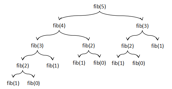
図I-1 フィボナッチ数を求める素朴な再帰関数のコールグラフ
図I-2 フィボナッチ数計算における計算の重複
    fib_pair(n) = [fib(n), fib(n-1)]                              (2)

        ここで [a, b] は a と b の組を表すものとする.
fib_pair(n-1) = [fib(n-1), fib(n-2)] (3)
    fib(n) = u where [u, v] = fib_pair(n)                         (4)
    fib_pair(n) = if n = 0 or n = 1 then [1, 1]
                  else [u + v, u]
                      where [u, v] = fib_pair(n-1)
                  end

        ここで Exp1(x) where x = Exp2 は,まず,式 Exp2 を計算して,その
	結果を x として,その上で式 Exp1(x) を評価することを表す.
        Exp1(x) の x は,式 Exp1 が変数 x に依存していることを表す意図で
        書いている.
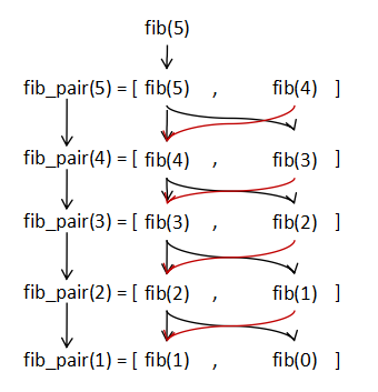
図I-3 フィボナッチ数の計算の重複の除去
fib_pair(n-1) = [fib(n-1), fib(n-2)] (3)
n に対する fib を求めるためには n-1 と n-2 に対する fib が求まって入れば良い.
知り合いの

私はもともと scheme のプログラムはあまり書いたことが無いうえに, 今回書くのは20~30年ぶりくらいなので,scheme プログラムとしてはあまり うまい表現ではないかもしれません. 一応,Windows 10 上に, Racket という処理系をインストールして動作を確かめました. 以下で実現した関数の意味は次の通りです.
以下は,結果を表示せず,再帰呼び出しの回数だけを返します.どの位計算に時間がかかっているかを確かめるための関数です.bar4, bar5 は n に 100 とか 1000 を
入れても大丈夫ですが,bar1, bar2, bar3 は,20 位にとどめておいてください.
うちの計算機はメモリーを 4GB 積んでいて,そこらあたりから少しずつ動作に
時間がかかるようになり,22, 23 では途中で止める必要がありました.計算機によっては,それ以下でも苦しいかも
しれませんので,
;;; 普通のハノイの塔のプログラム (define count1 0) (define (hanoi n a b c) (set! count1 0) (hanoi1 n a b c)) (define (hanoi1 n a b c) (begin (set! count1 (+ count1 1)) (if (= n 0) '() (append (hanoi1 (- n 1) a c b) (cons (list "Move" n "from" a "to" b) (hanoi1 (- n 1) c b a)))))) ;;; メモ化して同じ式を再計算しないようにしたハノイの塔のプログラム (define data2 '()) (define count2 0) (define (hanoi2 n a b c) (begin (set! count2 0) (set! data2 '()) (hanoi2b n a b c))) (define (hanoi2b n a b c) (let ((r (assoc (list n a b c) data2))) (set! count2 (+ count2 1)) (if (pair? r) (cdr r) (begin (if (= n 0) (set! r '()) (set! r (append (hanoi2b (- n 1) a c b) (cons (list "Move" n "from" a "to" b) (hanoi2b (- n 1) c b a))))) (set! data2 (cons (cons (list n a b c) r) data2)) r)))) ;;; プログラム変換 (タプリング戦略) で重複計算を除去した ;;; ハノイの塔のプログラム (define count3 0) (define (hanoi3 n a b c) (begin (set! count3 0) (car (hanoi3_triple n a b c)))) ;;; (hanoi3_triple n a b c) は意味的には ;;;(list (hanoi n a b c) (hanoi n b c a) (hanoi n c a b)) ;;; を返す関数.これを自分を参照する再帰関数に書き直す (define (hanoi3_triple n a b c) (begin (set! count3 (+ count3 1)) (if (= n 0) '(() () ()) (let ((x (hanoi3_triple (- n 1) a c b))) (list (append (car x) (cons (list "Move" n "from" a "to" b) (cadr x))) (append (caddr x) (cons (list "Move" n "from" b "to" c) (car x))) (append (cadr x) (cons (list "Move" n "from" c "to" a) (caddr x))) ))))) ;;; メモ化して同じ式を再計算しないようにしたハノイの塔のプログラム ;;; さらにリストの append を list で代用 (define data4 '()) (define count4 0) (define (hanoi4 n a b c) (begin (set! count4 0) (set! data4 '()) (hanoi4b n a b c))) (define (hanoi4b n a b c) (let ((r (assoc (list n a b c) data4))) (set! count4 (+ count4 1)) (if (pair? r) (cdr r) (begin (if (= n 0) (set! r '()) (set! r (list (hanoi4b (- n 1) a c b) (list "Move" n "from" a "to" b) (hanoi4b (- n 1) c b a)))) (set! data4 (cons (cons (list n a b c) r) data4)) r)))) ;;; プログラム変換 (タプリング戦略) で重複計算を除去したハノイの塔のプログラム ;;; さらにリストの append を list で代用 (define count5 0) (define (hanoi5 n a b c) (begin (set! count5 0) (car (hanoi5_triple n a b c)))) ;;; (hanoi5_triple n a b c) は意味的には ;;;(list (hanoi n a b c) (hanoi n b c a) (hanoi n c a b)) ;;; を返す関数.これを自分を参照する再帰関数に書き直す (define (hanoi5_triple n a b c) (begin (set! count5 (+ count5 1)) (if (= n 0) '(() () ()) (let ((x (hanoi5_triple (- n 1) a c b))) (list (list (car x) (list "Move" n "from" a "to" b) (cadr x)) (list (caddr x) (list "Move" n "from" b "to" c) (car x)) (list (cadr x) (list "Move" n "from" c "to" a) (caddr x))))))) ;;; それぞれのハノイの塔のプログラムを走らせるためのプログラム ;;; n に大きな数を与えると巨大な解を表示するので,小さい数だけで ;;; 試して,大きな数に対しては次の barN を使うこと (define (foo1 n) (hanoi n "A" "B" "C")) ;;; 普通のハノイの塔 (define (foo2 n) (hanoi2 n "A" "B" "C")) ;;; メモ化版 (define (foo3 n) (hanoi3 n "A" "B" "C")) ;;; タプリング版 (define (foo4 n) (hanoi4 n "A" "B" "C")) ;;; メモ化 + append サボり版 (define (foo5 n) (hanoi5 n "A" "B" "C")) ;;; タプリング + append サボり版 ;;; 結果を表示せず再帰呼び出しの回数のみを表示 (define (bar1 n) (begin (hanoi n "A" "B" "C") count1)) (define (bar2 n) (begin (hanoi2 n "A" "B" "C") count2)) (define (bar3 n) (begin (hanoi3 n "A" "B" "C") count3)) (define (bar4 n) (begin (hanoi4 n "A" "B" "C") count4)) (define (bar5 n) (begin (hanoi5 n "A" "B" "C") count5))
計算機(主にソフトウェア)の話題 へ
圏論を勉強しよう へ
束論を勉強しよう へ
半群論を勉強しよう へ
ホームページトップ(Top of My Homepage)